Beyond Row Stores: Columnar Storage, MPP Execution, and Distribution Design on Amazon Redshift vs. Amazon RDS for PostgreSQL

A technical deep dive into why analytical workloads need different database architecture. This article covers row-oriented vs. columnar storage, zone maps and compression encodings, MPP query execution, and distribution and sort key design. It also covers a controlled 20-million-row benchmark of RDS for PostgreSQL vs. Redshift, and AWS reference architectures using zero-ETL, DMS, Glue, and S3.

Muhammad Safiullah Khan

I code, travel, and build tech communities.

Published Oct 12, 2026

Last modified Oct 12, 2026

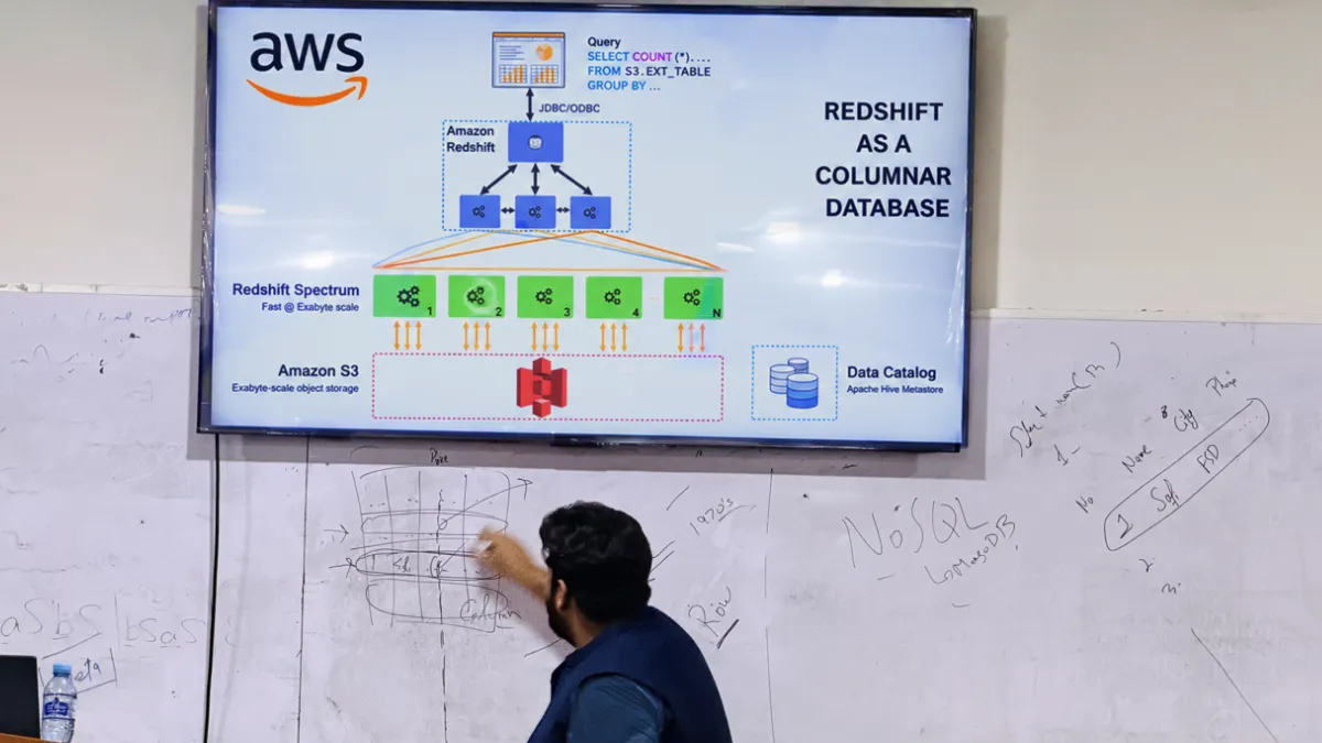
Author's note: This article expands on a technical session delivered on September 30 at COMSATS University Islamabad, Sahiwal Campus, hosted by the Computer Science Society CUI Sahiwal and the AWS Student Builder Group – CUI Sahiwal.

Abstract

Modern data platforms serve two fundamentally different workloads: transactional processing, where correctness and low-latency record-level operations dominate, and analytical processing, where queries scan, join, and aggregate millions or billions of rows. A database engineered for one is rarely optimal for the other. This article examines why, tracing the differences from the storage layout on disk through the query execution pipeline to distributed data placement. It then applies those principles to two AWS services, Amazon RDS for PostgreSQL and Amazon Redshift, describes a rigorous methodology for benchmarking them on a 20-million-row dataset, and closes with reference architectures for combining both services in a production AWS data platform.

1. OLTP and OLAP: Two Workloads, Two Design Centers

Online Transaction Processing (OLTP) systems handle high-concurrency, short-lived operations: inserts, updates, deletes, and point lookups by primary key. Their design priorities are ACID guarantees, MVCC-based concurrency control, B-tree indexing, and fast access to individual records. Typical access patterns touch a handful of rows and all of their columns.

Online Analytical Processing (OLAP) systems handle the inverse: queries that touch a very large number of rows but only a few columns, such as scans, aggregations, window functions, and multi-table joins. Typical latency targets are seconds, not milliseconds, but the data volumes involved are orders of magnitude larger.

Dimension	OLTP	OLAP
Primary operation	Point reads, single-row writes	Large scans, aggregations, joins
Rows touched per query	1 to hundreds	Millions to billions
Columns touched per query	Most or all	A small subset
Concurrency profile	Thousands of short sessions	Fewer, heavier queries
Storage orientation	Row-oriented	Column-oriented
Scaling model	Vertical, plus read replicas	Horizontal (MPP)
AWS service	Amazon RDS / Aurora	Amazon Redshift

Consider a query that computes total revenue by product category across 20 million order records. A row store must read every page that contains qualifying rows, and each page carries columns the query never references. An analytical engine can instead restrict I/O to exactly the columns the computation needs.

The distinction is therefore not about database size. It is about how data is stored, accessed, processed, and distributed to match the dominant workload.

2. Storage Internals: Row Heap vs. Columnar Blocks

2.1 PostgreSQL: row-oriented heap storage

Amazon RDS for PostgreSQL uses the standard PostgreSQL storage engine. Tables are stored as heap files divided into 8 KB pages, and each page holds complete tuples. Large values are moved out of line through TOAST. This layout is ideal for OLTP: fetching one customer record, or updating one order row, touches one or two pages. Index access paths (B-tree, GIN, BRIN) complement the heap by locating those pages quickly.

The cost appears on analytical scans. Aggregating three columns from a six-column table still pulls entire tuples through the buffer pool. The wider the table, the larger the share of wasted I/O.

2.2 Amazon Redshift: columnar storage

Amazon Redshift stores each column separately, in sorted, compressed blocks. Redshift RA3 instances and Redshift Serverless use Redshift Managed Storage (RMS), which keeps hot data on local SSD and persists data durably to Amazon S3, decoupling storage from compute so each can scale independently.

Given this schema:

1
2
3
4
5
6
7
8
CREATE TABLE orders (

    order_id         BIGINT,

    customer_id      BIGINT,

    product_category VARCHAR(64),

    quantity         INTEGER,

    unit_price       DECIMAL(10,2),

    order_timestamp  TIMESTAMP

);

the revenue-by-category query needs only three columns:

1
2
3
4
5
SELECT product_category,

       SUM(quantity * unit_price) AS revenue

FROM   orders

WHERE  order_timestamp >= DATE '2025-01-01'

GROUP  BY product_category;

Redshift reads blocks for product_category, quantity, unit_price, and order_timestamp only. The order_id and customer_id columns are never read. Three further mechanisms amplify the benefit:

Zone maps. Redshift records the minimum and maximum value of each 1 MB block. When a predicate falls outside a block's range, the whole block is skipped without being read. Zone maps are most effective when the filtered column is a sort key, because sorted data produces tight, non-overlapping ranges.
Vectorized, compiled execution. Redshift compiles query segments into machine code and processes data in column batches, which improves CPU cache utilization compared with tuple-at-a-time execution.
Block-level compression (covered next), which shrinks the bytes read from storage.

Columnar storage is not universally superior. Reconstructing a full row from many column files is expensive, and single-row updates are costly. Row stores remain the correct choice for transactional access patterns.

3. Compression: Reducing Analytical I/O

Compression is one of the largest contributors to columnar performance. Because values within a column share a type and often a similar distribution, they compress far better than heterogeneous values packed into rows.

Common techniques in analytical engines include:

Dictionary encoding: replaces repeated values with compact dictionary references. Highly effective for low-cardinality columns such as product_category.
Run-length encoding (RLE): stores consecutive repeated values as a (value, count) pair. Most effective on sorted columns.
Bit packing: stores integers in the minimum number of bits their range permits.
Delta encoding: stores differences between successive values. Well suited to timestamps and monotonically increasing identifiers.

Amazon Redshift exposes these as column encodings, including AZ64 (an AWS-designed encoding for numeric, date, and timestamp types), ZSTD, LZO, BYTEDICT, RUNLENGTH, DELTA, and RAW. In most deployments, the recommended approach is to let Redshift manage encodings automatically (ENCODE AUTO), or to run ANALYZE COMPRESSION to inspect recommendations on an existing table.

1
2
3
4
5
6
7
-- Inspect recommended encodings for an existing table

ANALYZE COMPRESSION orders;



-- Review current encodings and table health

SELECT "table", encoded, diststyle, sortkey1, size, tbl_rows, pct_used

FROM   svv_table_info

WHERE  "table" = 'orders';

Compression is not free. Effectiveness depends on cardinality, value distribution, sort order, and query patterns, and decompression consumes CPU. Whether it improves end-to-end latency must be validated against the full execution plan rather than assumed.

4. Distributed Query Execution in Amazon Redshift

Analytical performance depends on more than storage format. Execution architecture determines how efficiently stored data becomes a result.

4.1 The MPP architecture

A Redshift cluster consists of a leader node and one or more compute nodes. The leader node parses SQL, builds the plan, compiles code, and coordinates execution. Each compute node is divided into slices, each with dedicated memory and disk allocation, and each processing its portion of the data in parallel. In Redshift Serverless, compute capacity is expressed in Redshift Processing Units (RPUs) and provisioned automatically, but the same MPP execution model applies.

4.2 Stages of an analytical query

Parsing and planning. The leader node parses the SQL and the cost-based optimizer selects an execution strategy using table statistics.
Scan and projection. Compute nodes read only the required column blocks, using zone maps to skip irrelevant blocks.
Predicate evaluation. Filters are applied as early as possible so that non-qualifying data is excluded from later stages.
Partial aggregation. Each slice computes intermediate aggregates locally.
Data redistribution. When a join or aggregation requires co-located data, rows are redistributed or broadcast between nodes. This is typically the most expensive stage in a distributed plan.
Final aggregation and result delivery. Intermediate results are merged at the leader node and returned to the client.

4.3 Distribution styles

The distribution style determines which slice stores each row, and therefore how much network movement joins require.

Style	Behavior	Best for
`AUTO`	Redshift chooses and adjusts the style as the table grows	Default; recommended starting point
`KEY`	Rows with the same key value land on the same slice	Large fact and dimension tables joined on a common column
`ALL`	A full copy of the table on every node	Small, slowly changing dimension tables
`EVEN`	Round-robin distribution	Tables not involved in joins, or without a clear join key

When two large tables are joined on their distribution keys, the join can execute locally on each slice with no redistribution. A poorly chosen distribution forces a network shuffle. The EXPLAIN output exposes this through labels such as DS_DIST_NONE (no movement, ideal), DS_DIST_ALL_NONE, DS_BCAST_INNER (broadcast the inner table), and DS_DIST_BOTH (redistribute both sides, the most expensive).

4.4 Sort keys

Sort keys define the physical ordering of rows on disk. A compound sort key is best when queries filter on a leading prefix of the key columns. An interleaved sort key gives equal weight to each column but carries higher maintenance cost and is used less often today. For time-series fact tables, a timestamp or date column as the leading sort key is the standard pattern, since it maximizes zone-map pruning for range filters.

4.5 Automatic optimization features

Redshift reduces manual tuning through several managed capabilities. Automatic Table Optimization (ATO) can adjust distribution and sort keys based on observed workload. Automatic vacuum and automatic analyze maintain sort order and statistics. Materialized views with auto-refresh precompute expensive aggregations, result caching serves repeated identical queries without re-execution, and Concurrency Scaling adds transient capacity to absorb query spikes.

5. Amazon RDS for PostgreSQL vs. Amazon Redshift

Both services are managed, both speak SQL, and Redshift's SQL dialect is derived from PostgreSQL. Their architectures, however, target different problems.

Characteristic	Amazon RDS for PostgreSQL	Amazon Redshift
Primary use	OLTP, operational and mixed workloads	OLAP, data warehousing, BI
Storage model	Row-oriented heap, 8 KB pages	Columnar, compressed blocks
Execution model	Single-node, process-per-connection, limited intra-query parallelism	Distributed MPP, parallel across slices
Indexing	B-tree, GIN, GiST, BRIN	Sort keys and zone maps; no traditional secondary indexes
Scaling	Vertical scaling plus read replicas	Add nodes, RA3 managed storage, or Serverless RPUs
Transaction profile	High-concurrency short transactions, strong row-level semantics	Batch loads and large reads; not designed for high-frequency single-row writes
Bulk ingestion	`COPY` or `INSERT`	`COPY` from Amazon S3, parallelized across slices
Data lake access	Via extensions and tooling	Redshift Spectrum queries data in Amazon S3 in place

PostgreSQL can parallelize some scans and aggregates within a query, and a well-indexed PostgreSQL instance handles modest analytical workloads effectively. Redshift's advantage emerges as data volume and query complexity grow: its design assumes that scans and aggregations over large datasets are the normal case, not the exception.

The right choice depends on workload characteristics, concurrency, data volume, latency requirements, operational constraints, and cost, not merely on which database returns a result faster in a single test.

6. Experiment: Benchmarking 20 Million Records

To ground the concepts above, the session loaded 20 million records into both Amazon RDS for PostgreSQL and Amazon Redshift and ran analytical queries against each. The value of such an experiment depends entirely on how carefully it is controlled. A benchmark that compares a tuned system against an untuned one demonstrates configuration, not architecture.

6.1 Methodology

Identical data and semantics. Same schema, data types, row counts, and logical query results on both systems.
Fair physical design. On PostgreSQL, create appropriate indexes (B-tree on filter columns, or BRIN on the timestamp for append-only data) and run ANALYZE. On Redshift, choose suitable distribution and sort keys, allow encodings to be applied, and run ANALYZE.
Separate load from query time. Record ingestion duration independently from query latency.
Control caching. Redshift result caching will return near-instant results for repeated queries unless disabled for the session. On PostgreSQL, distinguish cold-cache from warm-cache runs.
Repeat and report distributions. Execute each query multiple times and report median and p95 latency, not a single run.
Document the environment. Record instance class and storage type (RDS), node type and count or base RPU capacity (Redshift), concurrency, and the exact SQL.

1
2
-- Redshift: disable result cache for the benchmarking session

SET enable_result_cache_for_session TO off;

6.2 Loading data efficiently

Bulk ingestion differs sharply between the two engines. In Redshift, loading from Amazon S3 with COPY parallelizes across slices, and splitting input into multiple compressed files of similar size improves throughput:

1
2
3
4
COPY orders

FROM 's3://my-bucket/orders/'

IAM_ROLE 'arn:aws:iam::123456789012:role/RedshiftCopyRole'

FORMAT AS PARQUET;

Row-by-row INSERT statements into Redshift are strongly discouraged for bulk loads because they bypass this parallelism.

6.3 Query workload

A representative benchmark set should span several query shapes rather than one favorable aggregation:

Full-scan aggregation: revenue by product category across all 20 million rows.
Filtered range aggregation: the same, restricted by order_timestamp to a narrow window.
High-cardinality group-by: aggregation by customer_id.
Join with aggregation: orders joined to a customer or product dimension table.
Point lookup: fetch one order by order_id, included deliberately to show where the row store wins.

Including the point lookup is important. An honest benchmark shows the trade-off in both directions.

6.4 Inspecting execution plans

On PostgreSQL, examine real execution behavior with:

1
2
3
4
EXPLAIN (ANALYZE, BUFFERS)

SELECT product_category, SUM(quantity * unit_price)

FROM   orders

GROUP  BY product_category;

Look for sequential versus index scans, parallel workers, buffer hits versus reads, and sorts or hash aggregates spilling to disk (governed by work_mem). On Redshift, use EXPLAIN to review distribution labels, then query system views for runtime detail:

1
2
3
4
5
6
7
8
9
10
11
EXPLAIN

SELECT product_category, SUM(quantity * unit_price)

FROM   orders

GROUP  BY product_category;



-- Query-level execution metrics (Redshift provisioned and Serverless)

SELECT query_id, elapsed_time, queue_time, execution_time,

       returned_rows, scanned_rows

FROM   sys_query_history

ORDER  BY start_time DESC

LIMIT  20;

7. Reference Architecture: Combining RDS and Redshift on AWS

In production, RDS for PostgreSQL and Amazon Redshift are complementary rather than competing. Running heavy analytical scans on the operational database degrades transactional latency and risks impacting customer-facing applications. Separating the workloads provides isolation and lets each tier be scaled and tuned independently.

7.1 Pattern A: zero-ETL integration

AWS offers zero-ETL integrations that replicate data from supported operational databases, such as Amazon Aurora and Amazon RDS engines, into Amazon Redshift with minimal pipeline code and low latency. This is the lowest-operational-overhead option when near-real-time analytics on operational data is the goal. Support varies by engine and version, so verify the current compatibility matrix in the AWS documentation before committing to this design.

7.2 Pattern B: S3-centered data lake pipeline

When you need raw data retention, multiple downstream consumers, or complex transformations, an S3-centered pipeline is more flexible:

Source: Amazon RDS for PostgreSQL holds operational data.
Extract: AWS Database Migration Service (AWS DMS) performs full load plus change data capture (CDC) into Amazon S3, typically as Parquet.
Store: Amazon S3 serves as the durable landing and staging layer, partitioned by date.
Transform: AWS Glue (ETL jobs and the Data Catalog) cleans and models the data.
Serve: Amazon Redshift loads curated data with COPY, or queries it in place through Redshift Spectrum.
Consume: Amazon QuickSight, SQL clients, and downstream applications query Redshift.

For streaming sources, Amazon Data Firehose can deliver event data directly into S3 or Redshift, and Redshift also supports streaming ingestion from Amazon Kinesis Data Streams and Amazon MSK.

7.3 Choosing between the patterns

Requirement	Recommended approach
Near-real-time analytics, minimal pipeline maintenance	Zero-ETL integration
Raw data retention, multiple consumers, complex transformation	S3 data lake with DMS and Glue
Event or clickstream ingestion	Firehose, Kinesis, or MSK into S3 or Redshift
Occasional queries on cold or archival data	Redshift Spectrum over S3

The correct design depends on data freshness requirements, volume, transformation complexity, governance, security, and cost.

7.4 Operational considerations

Security: encrypt at rest with AWS KMS and in transit with TLS; control access with IAM roles and, for Redshift, role-based access control; keep clusters in private subnets within a VPC.
Cost management: compare Redshift provisioned (RA3, with reserved capacity for steady workloads) against Serverless (usage-based, suited to variable workloads); apply S3 lifecycle policies to staging data.
Monitoring: use Amazon CloudWatch and RDS Performance Insights for the operational tier, and Redshift system views and query monitoring rules for the warehouse.
Table maintenance: keep statistics current, review skew and distribution with svv_table_info, and revisit design as query patterns evolve.

Key Takeaways

OLTP and OLAP are different design centers. Row stores optimize for retrieving and modifying whole records; columnar stores optimize for scanning a few columns across many records.
Columnar storage plus compression reduces I/O. Zone maps and sort keys let Redshift skip data entirely, not just read it faster.
Distribution design drives distributed performance. Minimizing data redistribution through sound distribution and sort key choices is often the single largest lever in a Redshift workload.
Benchmark honestly. Control caching, tune both systems fairly, repeat runs, report percentiles, and include workloads where the row store wins.
Use both services together. Keep RDS for PostgreSQL as the system of record and offload analytics to Redshift through zero-ETL or an S3-centered pipeline.

Snapshots from the Workshop

The session at COMSATS University Islamabad, Sahiwal Campus, was built around live interaction rather than slides alone. Students followed the architecture discussion, from row-oriented heap pages to columnar blocks and MPP execution, and then watched the same analytical queries run against the 20-million-row datasets on Amazon RDS for PostgreSQL and Amazon Redshift. Comparing execution plans side by side turned abstract concepts such as zone maps, distribution styles, and data redistribution into something visible, and it prompted practical questions about indexing, sort keys, and when each service is the right choice.

Conclusion

Choosing a database requires understanding the workload and the architecture behind the SQL interface. Storage layout, compression, query optimization, parallel execution, and data distribution all shape analytical performance, and AWS provides purpose-built managed services for each side of the workload spectrum. Engineers who understand why these systems behave differently are better equipped to design platforms that are fast, scalable, and cost-effective.

My thanks to the Computer Science Society CUI Sahiwal and the AWS Student Builder Group – CUI Sahiwal for the opportunity to share practical engineering knowledge with students passionate about databases, cloud computing, and data engineering.

#AWS #AmazonRedshift #AmazonRDS #PostgreSQL #OLAP #DataEngineering #ColumnarDatabases #AWSCommunity #CloudArchitecture

# amazon-redshift # amazon-rds # data-warehouses # analytics # aws-workshops

Any opinions in this article are those of the individual author and may not reflect the opinions of AWS.

Enjoyed reading this content? Let the author know!

Your likes, comments, shares, and saves help creators reach more builders.

Loading recommendations

Loading article

Builder Center

Beyond Row Stores: Columnar Storage, MPP Execution, and Distribution Design on Amazon Redshift vs. Amazon RDS for PostgreSQL

Muhammad Safiullah Khan

Abstract

1. OLTP and OLAP: Two Workloads, Two Design Centers

2. Storage Internals: Row Heap vs. Columnar Blocks

2.1 PostgreSQL: row-oriented heap storage

2.2 Amazon Redshift: columnar storage

3. Compression: Reducing Analytical I/O

4. Distributed Query Execution in Amazon Redshift

4.1 The MPP architecture

4.2 Stages of an analytical query

4.3 Distribution styles

4.4 Sort keys

4.5 Automatic optimization features

5. Amazon RDS for PostgreSQL vs. Amazon Redshift

6. Experiment: Benchmarking 20 Million Records

6.1 Methodology

6.2 Loading data efficiently

6.3 Query workload

6.4 Inspecting execution plans

7. Reference Architecture: Combining RDS and Redshift on AWS

7.1 Pattern A: zero-ETL integration

7.2 Pattern B: S3-centered data lake pipeline

7.3 Choosing between the patterns

7.4 Operational considerations

Key Takeaways

Snapshots from the Workshop

Conclusion