
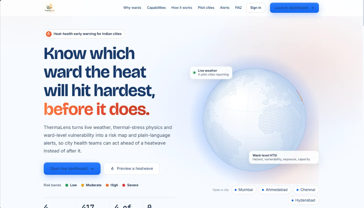
Building ThermaLens: Ward-Level Heat Intelligence for Indian Cities on AWS
How we combined thermal-stress physics, Census data and satellite imagery into a ward-by-ward heat-risk map, ran it on AWS Elastic Beanstalk, and learned where the prototype still falls short. By Team Murf-guys · Bharat Builds Tour × WeMakeDevs × AWS

Building ThermaLens: Ward-Level Heat Intelligence for Indian Cities on AWS
How we combined thermal-stress physics, Census data and satellite imagery into a ward-by-ward heat-risk map, ran it on AWS Elastic Beanstalk, and learned where the prototype still falls short.
By Team Murf-Guys· Bharat Builds Tour × WeMakeDevs × AWS
Two wards in the same city can receive the same heat warning and live through very different afternoons. One has tree cover, a hospital nearby and homes with air conditioning. The other has bare concrete roofs, dense housing and a high share of elderly residents. A city-wide forecast treats them identically.
We built ThermaLens (Thermal Assessment & Protection Analytics System) to see what it would take to tell them apart. The goal was not a more precise temperature. It was to connect heat, local environment and population vulnerability at the scale where municipal teams actually make decisions.
The hard part turned out not to be computing a score. It was building something that could show where its inputs came from, say what it did not know, and keep working when data was missing.

Figure 1. The city view for Ahmedabad: every ward is coloured by its risk band, and a layer switcher moves between risk, modelled mortality, modelled hospitalisation, UTCI and vegetation.
This is the dashboard as it runs today. The rest of the article explains what sits behind that map.
Why air temperature is not enough
Extreme heat is both a public-safety and a planning problem. Warnings in many places are issued at district or city scale and lean heavily on air temperature. That leaves two gaps.
The first is spatial. Within a city, built density, vegetation, housing quality and access to cooling vary from ward to ward, and those differences shape who is exposed and who can cope.
The second is physiological. The body does not respond to air temperature alone. Humidity limits how well sweat evaporates, wind carries heat away, and sunshine adds radiant load. ThermaLens therefore uses the Universal Thermal Climate Index (UTCI) , which folds temperature, humidity, wind and radiation into a single "feels-like" figure. We compute it with the
pythermalcomfort Python library.A score on a map is not yet a response, though. So each ward's band is paired with recommended actions for administrators, and with plain-language guidance for residents in English, Hindi and the state language of each pilot city.
What we built
ThermaLens covers four pilot cities (Mumbai, Ahmedabad, Chennai and Hyderabad), which the repository documents as 417 wards in total. Navigation runs India → city → ward. In a city view you switch layers, select a ward and see its four risk factors, its five-day outlook and its recommended actions. Planning tools let you preview a hotter day, test preventive measures and rank wards for resources.
Two caveats belong up front. The Hyderabad boundaries (144 wards) come from the corporation's earlier layout, which has since been reorganised. And most vulnerability indicators come from Census 2011. ThermaLens's ward-level numbers are modelled estimates, not measurements.
The architecture
ThermaLens separates slow-moving inputs from fast-moving ones. Ward geometry, climatology, Census tables and satellite-derived features are prepared ahead of time and shipped with the application. Weather is fetched live. The FastAPI backend merges the two, scores every ward, serves
the dashboard and runs a scheduler for alerts.
the dashboard and runs a scheduler for alerts.

Figure 2. System architecture. In the deployed environment, data lives in container-local JSON files. PostGIS is an optional path, and S3 is not part of the runtime.
Read the diagram from the top. Two kinds of input enter the container: live forecasts through the ingestion module, and prepared datasets loaded from files. The risk engine joins them. Its results flow two ways: to the API and map for people to explore, and to the scheduler, which decides whether any ward has crossed into a band that warrants an alert.
A page load asks for static ward geometry once, which the browser caches, and then for city and ward results from a snapshot cache that lasts 15 minutes. A weather refresh happens on the scheduler. It re-fetches forecasts, rescores all 417 wards, and checks for escalations.
Where the numbers come from
Not every input is equally live, and we try to say which is which.
| Class | Examples | How it is used |
|---|---|---|
| Live | OpenWeatherMap 5-day, 3-hour forecast | Refreshed on a schedule |
| Prepared (static) | ERA5 climatology via Open-Meteo (2014–2024), MODIS land-surface temperature and NDVI, WUDAPT Local Climate Zones, Census 2011 and HL-14, OpenStreetMap hospitals and ward boundaries | Shipped with the app |
| Derived or estimated | Built, vegetation and water fractions from Esri imagery; solar radiation from a clear-sky model scaled by cloud cover | Flagged as estimates |
| Fallback | A labelled demonstration weather series | Used only when live data is unavailable |
The satellite-imagery fractions are a rough proxy, thresholded from true-colour imagery. They are not an official land-cover product, and we treat them that way.
Wards are snapped to a 0.028° grid, roughly 3 km, so wards in one cell share a weather record. That keeps us within the free-tier call budget, but it means weather resolution is coarser than the ward polygons.
When no API key is configured or a request fails, the system reuses the last good record for up to six hours. After that it falls back to the demonstration series, and the interface says which cities are on live and which on fallback. We chose that visible label over quietly filling the gap. A map that looks complete but hides its estimates is less trustworthy than one that shows its seams.
The model: HTSI
At the core is one expression:
1
HTSI = H × V × E × (1 − AC)
The idea is that risk needs four things at once. Heat has to be dangerous, people have to be susceptible, the environment has to trap heat, and cooling options have to be limited. If any of the first three is near zero, or capacity is high, the product falls.

- H, hazard. How abnormal and how physiologically stressful is the heat? We blend two signals:
H = 0.62·a + 0.38·surge. The anomalyais how far the day's maximum temperature sits above the city's monthly normal from ERA5. It rises from 0 at the normal, to 0.5 at +4.5 °C, to 1.0 at +6.4 °C, following IMD heatwave departure criteria. The surge is how far UTCI exceeds 36 °C, scaled over ten degrees. We follow IMD thresholds but make no claim that the result is IMD-certified. - V, vulnerability. A seven-indicator index from Census data: children aged 0–6, literacy, slum share, residents over 60, disability, density and kutcha housing. Most of it is city-level, with kutcha housing taken per ward where HL-14 data matched.
- E, exposure. Built, vegetation and water fractions, adjusted by MODIS land-surface temperature and the LCZ built share.
- AC, adaptive capacity. A proxy for cooling access. It starts from a city baseline and shifts per ward with built density, greenery, electricity and tap-water access, and hospitals per square kilometre. It is a proxy, not survey data.
HTSI is banded into Low, Moderate, High and Severe at 0.055, 0.115 and 0.185.

Figure 3. The risk pipeline. Weather becomes hazard; hazard combines with the three static ward factors into HTSI and into two separate health-risk scores.
The same four factors also feed two logistic models that produce modelled mortality and hospitalisation scores. These are the part we are most careful about. Their coefficients are manually specified defaults, not fitted values. A calibration layer attaches a relative risk and labels its basis as fitted, published-anchor or default. Fitting requires at least 365 observed rows and 15 hot days. No local death or admission records are loaded, so the mortality component rests on a published relative-risk anchor and the hospitalisation component is uncalibrated.
These numbers are relative, modelled scores. They are not forecast probabilities that a person will die or be hospitalised. ThermaLens is a parametric geospatial model with logistic terms. It is not a trained machine-learning system.
The ward panel exists to make the model explain itself. Instead of showing a colour and nothing else, it shows how much each factor contributed, so an officer can tell whether a ward is high because of heat, population, built environment or lack of cooling.
From a score to something usable
A risk band only matters if it leads somewhere. The forecast panel shows the daily peak HTSI for five days, with each bar's opacity following a confidence value that drops with lead time: 1.0 within a day, 0.85 out to three days, 0.62 to four, 0.45 beyond.
- A preventive-measures simulator re-runs the model with raised adaptive capacity.
- A resource-allocation view ranks wards by modelled priority.
- A CSV export lists every ward's components for audit.
- A heatwave preview raises temperatures and labels every output PREVIEW everywhere, so a rehearsal can't be mistaken for an observation.
The effect sizes in the scenario tools are illustrative and unvalidated. They are for exploring options, not predicting results.
Alerts follow a lifecycle. When a ward escalates into High or Severe and its cooldown has passed (six hours for High, three for Severe), the system builds a message with the band, the thermal reading and guidance in English, Hindi and the state language, plus the emergency numbers 112 and 108. A six-hourly city digest skips wards that already received an individual alert.

Sending depends on configuration. With Twilio credentials the message goes through SMS or WhatsApp. Without them it is written to an outbox and labelled SIMULATED. We keep four states apart: generated, simulated, accepted by a provider and delivered. We haven't demonstrated the last, and the documented configuration targets a single configured recipient, not routing to residents.
Making the map the interface

The dashboard is built on MapLibre GL JS. The question ThermaLens asks is comparative, which wards stand out relative to their neighbours, and that is easier to answer on a map than in a table. The map offers Dark, Light, Satellite and Streets basemaps and a Flat or Raised view. Each layer carries its own legend, and the readout names whichever layer is active. Static ward geometry is fetched once per city and cached in the browser, so switching layers does not reload polygons.
We also added sign-up and a profile (location, age range and optional ailments, with explicit consent). In its current form this is storage only: it feeds an in-app alert preview, and it does not change the risk engine. The accounts are demo-grade, with PBKDF2 password hashing in a local file, and we don't present them as a production identity system.
How we run it on AWS
ThermaLens runs as a single Docker container on AWS Elastic Beanstalk in the Asia Pacific (Mumbai) Region. We chose a container because the same
Dockerfile that builds the image locally, optionally alongside PostGIS through Docker Compose, is what Elastic Beanstalk runs in the cloud. The geospatial and scientific Python dependencies behave the same in both places.Elastic Beanstalk is the deployment and environment manager. It takes an application version, provisions and manages the underlying Amazon EC2 instance, runs the container on the Docker platform on Amazon Linux 2023, and reports environment health. The EC2 instance is the compute that runs FastAPI and Uvicorn, the weather ingestion, the ward calculations and the scheduler.
The console's deployment history shows four events, all succeeded: environment creation, one configuration update, and two application deployments using the all-at-once policy. The environment reports health Ok and runs a single instance.

Figure 4. The ThermaLens environment in Elastic Beanstalk: healthy, on the Docker platform, with four successful deployment events.
For observability, Elastic Beanstalk streams its logs to Amazon CloudWatch. The environment has nine log groups with a seven-day retention period.

Figure 5. The hosting boundary. Solid arrows are running today. Dotted arrows show log delivery and one planned integration that does not exist yet.
The path in Figure 5 is a straight line from a source bundle to the public API. Beanstalk owns the environment and the instance, CloudWatch receives logs, and S3 is drawn dashed because the application does not use it.
| Component | Status |
|---|---|
| Elastic Beanstalk, Docker platform, managed EC2 | In use; health Ok |
| CloudWatch log streaming and 7-day retention | Configured |
| CloudWatch alarms | Not configured yet |
| S3 for application data | Planned; no adapter in the code |
| IAM least-privilege instance profile, secrets management | Not verified; treat as to-do |
Elastic Beanstalk itself keeps application versions in S3, but that is the platform's storage and not ours. Creating a bucket for ThermaLens would change nothing until the datastore gains an adapter, a bucket setting and an instance profile limited to the access it needs, with S3 Block Public Access left on. The demo is also served over plain HTTP. It is a working prototype, not a hardened public-safety service.
What fought back
A mild day that scored as a heatwave. Our first anomaly logic compared the day's maximum only against the monthly normal. A 33 °C day in Hyderabad in September, against a cool-season normal of 28.8 °C, scored as a heatwave. IMD criteria also require a hot absolute maximum, 40 °C on plains and 37 °C on the coast. We added a gate that scales positive anomalies by how close the day's maximum is to that threshold. Our first version used a hard zero, and it flattened every ward's hazard to nothing on cooler days, erasing the ranking between wards. We settled on a floor of 0.25. The ramp width and floor are unvalidated, and "coastal" is a hard-coded list of two cities. A residual limit remains: if the anomaly is zero or negative and UTCI is below 36, hazard is still zero by construction, so on a genuinely cool day every ward reads Low.
Static terms that never switched off. Exposure, vulnerability and cooling access apply all year, so a dense, low-cooling ward could read High in December. We added a seasonal factor between 0.25 and 1.0 based on how close the month's normal temperature is to the city's hottest month. It scales only those three static terms, never the live hazard terms, and a strong anomaly or a UTCI near 44 overrides it. The result is a smooth heuristic that doesn't model monsoon versus winter, and its floor is unvalidated.
A quota that shapes the design. On OpenWeatherMap's free tier we budget calls: 55 per minute, a monthly limit with a planned share, a clamped refresh interval (30 minutes by default), and grid snapping so nearby wards share a record. The national rescore runs only when weather actually refreshes. The trade-off is that a change to model weights does not show up until the next refresh, and weather resolution is coarser than the ward map implies. One input is also filled in silently: relative humidity defaults to 50% when it's missing, at odds with our own preference for visible gaps.
Data that ages, and state that doesn't persist. Hyderabad's boundaries and the Census inputs are dated, which limits how much weight any ward-level difference can bear. Separately, the application writes users, weights and the alert outbox to files inside the container. We haven't mounted a volume or added object storage for them, so they would not necessarily survive the replacement of an instance. Health checks and logs tell us the app is running. They tell us nothing about whether its data will survive. This is the clearest gap between "deployed" and "durable".
Testing and what we can claim
The test suite runs offline with the scheduler disabled. It covers the seasonal factor, the IMD gate, a regression test against all-zero HTSI, API behaviour and alert construction. At the last documented run, 56 tests passed and one failed. The failing test expected a value from the symmetric-anomaly formula that the code does not produce, so either the test or the formula needs updating.
It helps to separate four things. ThermaLens is a working software pipeline. It generates model outputs from inputs. It is not a model calibrated on sufficient local observations, and it has not been validated against independent real-world outcomes. We have no local health data to test against, so we make no claim about reduced mortality or admissions.
One presentation detail follows from this. The dashboard currently formats the mortality and hospitalisation scores like percentages, which invites reading them as literal probabilities. Relabelling them as modelled scores is near the top of our list.
What comes next
Near-term engineering:
- Build and test a storage adapter, S3 or a database, for datasets, alert history and user data.
- Add CloudWatch alarms for unhealthy instances and elevated error rates.
- Fix the failing test.
- Relabel the health outputs.
Work that needs data, partners or institutions:
- Updated ward boundaries and demographic indicators.
- Real municipal death and admission records for calibration.
- Review of the model by public-health experts.
- Alert delivery with recipient routing, consent and delivery tracking.
- New cities, once their input data is prepared.
What we learned
Spatial resolution is only useful when the data justify it. Our ward polygons are fine-grained, but most vulnerability indicators are city-level, so many ward-to-ward differences come from the environmental layers.
A map should explain the model, not hide it. Showing four factors next to every score made disagreements with intuition easy to investigate.
Fallback behaviour is part of reliability. Labelling live, estimated and demonstration data matters as much as the calculation.
And a deployment is not a storage design. Beanstalk gave us a repeatable way to run the container and CloudWatch gave us logs. Neither made our data durable.
A city-wide warning will always be useful. Showing which wards sit behind it is the next step, and getting from a prototype to something a city can rely on takes data access, validation and operational work that we have only begun.
References
Project
- Code: https://github.com/yash565-git0/ThermaLens
- Live demo (HTTP): http://thermalens-env.eba-3r3dd5cq.ap-south-1.elasticbeanstalk.com/
AWS documentation
- AWS Elastic Beanstalk Developer Guide
- Docker platform for Elastic Beanstalk
- Streaming Elastic Beanstalk logs to CloudWatch
- Elastic Beanstalk instance profiles
- S3 Block Public Access
Data and science
- UTCI
- OpenWeatherMap 5-day forecast
- Open-Meteo historical weather API (ERA5)
- WUDAPT Local Climate Zone map, Demuzere et al. 2022 (Zenodo)
- MapLibre GL JS
- de Bont et al. 2024, Environment International 184:108461 (mortality relative-risk anchor; full citation and DOI to confirm)
Enjoyed reading this content? Let the author know!
Your likes, comments, shares, and saves help creators reach more builders.

Loading recommendations
Loading article