
WasteFlow AI: Planning Waste Collection Before the Bins Overflow
WasteFlow AI is a hackathon prototype that connects a machine-learning waste model, bin pickup priorities, fleet planning, and sustainability scenarios in one dashboard, built with Amazon SageMaker and Amazon S3. It runs on synthetic data, and this article is explicit about what is simulated, what works today, and what comes next.

Predict better. Plan smarter. Waste less.
Two bins, same city, same morning. One sits in a busy market and has been overflowing since noon. The other is in a quiet lane, half empty, and a truck is about to empty it because the schedule says so.
Nobody made a bad decision. The schedule was fixed, and nobody had an estimate of where waste would pile up.
WasteFlow AI is our hackathon answer to one question: what changes when waste collection is planned from data instead of habit? It connects four things that are usually handled separately: a machine-learning waste model, bin pickup priorities, fleet planning, and sustainability scenarios. All of it lives in one interactive dashboard, built for the Waste and Energy theme.
One thing up front: it runs on synthetic data. We say so wherever it matters, because a prototype earns trust by being clear about what it is.
At a glance
Item | Detail |
|---|---|
Theme | Waste and Energy |
What it is | A working prototype dashboard with a trained model and a FastAPI backend |
Data | Synthetic: about 219,000 daily records, 300 bins, five Delhi wards, 2018 to 2019 |
ML task | Predict daily waste per bin, in kilograms |
Test result | MAE 6.875 kg versus 14.913 kg for a simple baseline |
Built with | Amazon SageMaker Studio, Amazon S3, Python, FastAPI, HTML, CSS, JavaScript |
Status | Prototype. Not deployed in any city, no live sensors, no GPS |
The problem: three decisions made separately
Waste collection is not one decision. It is a chain of them, and each link usually lives in a different place. The same small inefficiencies then repeat every single day.
Question | Why it is hard today |
|---|---|
How much waste is coming? | Volumes shift by location and over time, so a flat average misses the peaks. |
Which bins need attention first? | Without estimates, teams visit bins by schedule, not by need. |
What will it take to move it? | Trucks, trips, and distance depend on volume, but volume is rarely linked to fleet planning. |
The usual result is overflow in some places, wasted trips in others, and fuel burned in between. And because generation, pickup, transport, and environmental impact are tracked in different places, it is hard to see the trade-offs between them.
The idea: connect the chain
Most tools handle one link. WasteFlow AI connects them: estimate waste, prioritise bins, size the fleet, and test the environmental consequences.
A waste estimate becomes useful when it changes a pickup priority. A pickup priority becomes useful when it informs truck demand. And truck demand becomes more meaningful when you can see its effect on emissions and landfill. The goal is not to replace a municipal team’s judgement. It is to let them explore decisions before committing trucks and crews.
How it fits the Waste and Energy theme
The scenario model covers several parts of the theme. These are assumption-based what-if levers, not measured results.
Theme area | How WasteFlow AI touches it |
|---|---|
Segregation | A “sorting at source” lever shows its effect on landfill diversion |
Recycling | Dry and mixed-waste recovery assumptions feed a recycling stream |
Informal recyclers | A waste-picker share lever shows the effect on truck load and distance |
E-waste | E-waste is modelled as its own stream to a dedicated facility |
Cutting what a city burns | Fleet choice (diesel, CNG, or electric) and distance driven change estimated CO2 |
Cleaner energy | Biogas plant output, electricity, and bio-CNG are estimated from organic waste |
Not covered | Rooftop solar and public transport |
Pipeline at a glance
Stage | What happens | Where |
|---|---|---|
1. Data | Synthetic daily waste records for 300 bins are stored | Amazon S3 |
2. Training | The model is trained on 2018 to mid-2019 and tested on mid-2019 to end-2019 | SageMaker JupyterLab |
3. Artifacts | model.joblib, evaluation_metrics.json, test_predictions.csv, fill_estimates.csv, collection_recommendations.csv | Saved to S3 |
4. API | FastAPI serves bins, recommendations, metrics, historical predictions, and scenarios | Uvicorn, port 8000 |
5. Dashboard | The web interface reads the API and runs scenario calculations | Port 8080 |
Built on AWS
Layer | Technology | Role |
|---|---|---|
Development | Amazon SageMaker Studio (JupyterLab) | Data preparation, model training, evaluation |
Storage | Amazon S3 | Datasets, trained model, output files |
Backend | Python, FastAPI, Uvicorn | Serves estimates, recommendations, metrics, historical predictions, scenarios |
Frontend | HTML, CSS, JavaScript | Interactive dashboard that reads from the API |
The model, the API, and the interface are separate, so a new data source can be connected later without rebuilding the dashboard.
Endpoint | Returns |
|---|---|
/bins and /bins/{bin_id} | Bin estimates and per-bin details |
/recommendations | Collection recommendation records |
/model-metrics | Model evaluation results |
/forecast-data | Historical test-period predictions |
/scenario | Scenario-based waste estimates |
We checked the API directly: the /bins endpoint returns 300 bin records, and every response is marked as simulated historical estimates.
The machine-learning pipeline
We generated a synthetic dataset of about 219,000 daily records covering 300 bins across five Delhi wards, from January 2018 to December 2019. We used synthetic data because verified municipal records were not available to us.
The model predicts daily waste per bin in kilograms. It does not predict live fill levels or track vehicles.
Set | Rows | Period |
|---|---|---|
Training | 163,800 | 1 Jan 2018 to 30 Jun 2019 |
Test | 55,200 | 1 Jul 2019 to 31 Dec 2019 |
Metric | Our model | Simple baseline |
|---|---|---|
MAE (average absolute error) | 6.875 kg | 14.913 kg |
RMSE (penalises large misses more) | 9.835 kg | 20.772 kg |
MAE tells you the typical size of a miss. RMSE punishes the big misses harder, so it is a stricter test. The model beats the baseline on both, and its typical daily error is less than half the baseline’s. Because the data is synthetic, these are preliminary prototype results. They show that the workflow works end to end, not how it would perform in a real city.
How we tried not to fool ourselves
- Chronological split. The test period comes after the training period, so the model is judged on data it never saw.
- A baseline to beat. A model only means something next to a simple alternative.
- No overclaiming. We report evaluation metrics as evaluation metrics, not as real-world accuracy.
From waste estimates to bin fill levels
The model predicts waste in kilograms, but a collection team thinks in full bins. So the backend converts predictions into estimated fill levels using two stated assumptions: a waste density of 0.15 kg per litre, and a collection threshold of 80% full. Bins above the threshold are flagged for pickup, and the results are saved as fill_estimates.csv and collection_recommendations.csv.
This is an estimate chain, not a measurement: predicted kilograms, then an assumed density, then an assumed capacity, then a fill percentage. That is why every bin figure in the interface is labelled as a simulated historical estimate.
Where each page gets its numbers
This is the part we most want judges to see, because it is easy to blur in a demo.
Page | Where the numbers come from |
|---|---|
Bins | Bin-level estimates from the FastAPI /bins endpoint (300 bins, five wards) |
Forecasts | Historical actual versus predicted waste from the model’s test period |
Dashboard, Trucks & Routes, AI Recommendations, Analytics, Alerts, Simulation, Live Map | An in-browser scenario engine on a calibrated demo city of 12 wards and 640 tonnes per day, driven by editable assumptions |
The scenario engine and the 300-bin dataset are two separate worlds. We kept them separate and say so, rather than pretending they are one integrated system.
What the dashboard does today
Page | What it shows | What it is not |
|---|---|---|
Bins | Estimated fill and pickup priority per bin | Not sensor readings |
Trucks & Routes | Six illustrative fleet groups with estimated trucks, trips, and distance | Not GPS tracking or an optimised road route |
AI Recommendations | Suggested changes, recalculated for the current scenario, which can be applied to the simulation | Not verified municipal outcomes |
Forecasts | Actual versus predicted waste for the synthetic test period, 18 to 31 December 2019 | Not a future forecast |
Analytics | Landfill diversion, CO2 avoided, distance driven, biogas electricity, versus a normal day | Not measured impact |
We renamed “Trucks on the road” to “Estimated trucks needed”, so a plan is never mistaken for tracking.
A closer look at the dashboard
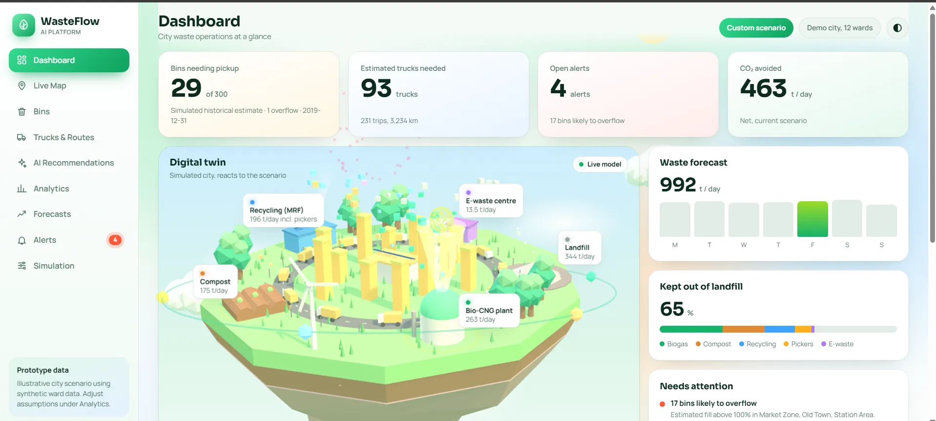
Dashboard. A “today at a glance” row shows estimated bins needing pickup, estimated trucks needed, open alerts, and CO2 avoided for the current scenario. A 3D view visualises the same flows, with wards as towers, facilities such as the biogas plant, compost site, recycling centre, e-waste centre, and landfill, and trucks circling the city. It is a visual aid driven by the same scenario numbers.
Flow diagram. A Sankey diagram traces waste from organic, dry recyclable, e-waste, and residual streams to the biogas plant, compost, recycling, waste pickers, the e-waste facility, and landfill. A mass-balance line checks that tonnes out equal tonnes in.
Alerts. Simple rules run on the current scenario and flag capacity and demand problems:
Alert | Triggered when |
|---|---|
Bins likely to overflow | Estimated fill is above 100% |
Biogas plant offline | The plant outage toggle is on |
Organic waste has no facility | Compost and biogas capacity are both full |
Plant or compost site near capacity | More than 90% of capacity is in use |
Heavy landfill share | More than half the waste still reaches landfill |
Truck demand up | Estimated trucks needed rise more than 20% above a normal day |
Live Map. Wards, bins, facilities, and trucks on one map, with layers you can switch on and off. Truck positions are simulated along a planned route, because there are no sensors. The interface states this on the page.
Route comparison. The Simulation page compares a fixed legacy stop order with a route improved by a 2-opt routine. This runs on 12 abstract ward positions, not real roads or coordinates, so it illustrates the idea of route optimisation rather than delivering a validated route.
Scenario analysis: decide before committing
Cities do not run on normal days. They run on festivals, monsoons, and equipment failures.
Users can compare a normal day against an alternative by changing waste uplift, sorting at source, the informal waste-picker share, fleet type, and plant availability. The dashboard includes presets for a normal day, Diwali week (+40% waste), Monsoon (+15%), and a biogas plant outage.
In one backend run, a reference prediction of about 9.5 tonnes for 31 December 2019 became about 13.3 tonnes under a 40% uplift assumption. That is a what-if on historical synthetic data, not a forecast of the future. The sorting input is recorded as a scenario parameter, and the backend does not claim that sorting causes less waste.
The scenario engine under the hood
Step | What the engine does |
|---|---|
1. Total waste | Starts from the demo city’s 640 tonnes per day, adjusted by the uplift |
2. Split | Divides waste into organic, dry recyclable, e-waste, and residual shares |
3. Recovery | Sorting at source raises how much of each stream reaches the right facility |
4. Facilities | Biogas and compost sites take organic waste up to their capacity limits, and the rest goes to landfill |
5. Fleet | Converts load into trips and trucks, using 4 tonnes per truck and 2.5 trips per truck per day |
6. Impact | Estimates biogas electricity and bio-CNG, fleet emissions, and CO2 avoided against a diesel baseline |
The truck and facility figures are demo constants that a real operator would replace with their own fleet and plant data.
Showing uncertainty, not false precision
The dashboard has an assumptions register with 17 editable entries, such as organic share, biogas yield, truck mileage, and emission factors. Each has a low, mid, and high value, and each is tagged as sourced, typical, or assumed. So the dashboard shows:
- likely ranges for key results, from 240 random draws across the low-to-high assumption ranges
- a sensitivity view of which assumptions move the CO2 estimate the most
- a mass-balance check that the tonnes going out of the system equal the tonnes coming in
Design principles
- Label everything honestly. Estimates say “estimated”. Historical data says “historical”. Simulated positions say “simulated”.
- Show the assumptions. If a number depends on an assumption, the user can see it and change it.
- Prefer ranges to single numbers. A confident-looking number hides uncertainty.
- Keep the parts separate. Model, API, and interface can each change without breaking the others.
Challenges we hit
Challenge | What we did |
|---|---|
Managed training was blocked: our ml.m5.large training quota was zero | Trained the model locally in SageMaker JupyterLab and saved the artifacts to S3 |
Estimates could be mistaken for live readings | Reworded labels and marked bin figures as simulated historical estimates |
The scenario engine uses a 12-ward demo city, separate from the 300-bin dataset | Kept the two clearly separate and documented the gap openly |
Serving the API and the dashboard from a cloud notebook environment | Ran them on separate ports and connected them through the notebook’s proxy URLs |
Keeping two copies of the frontend in sync | Made changes in one working copy at a time and checked JavaScript syntax after each change |
Enjoyed reading this content? Let the author know!
Your likes, comments, shares, and saves help creators reach more builders.

Loading recommendations
Loading article