
BreatheAhead: Exploring Smoke Pathways with Satellite Data and AWS
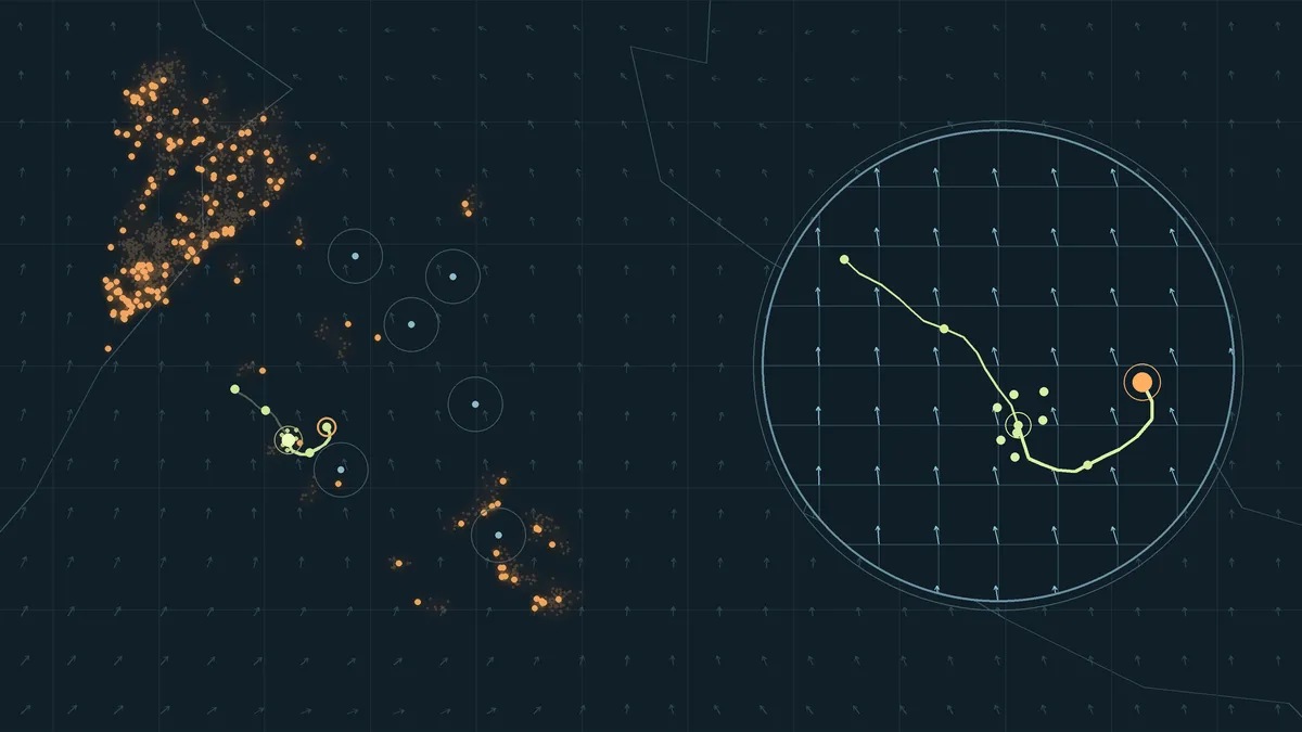
I built an interactive map that combines real satellite detections and wind data to explore potential smoke transport across northern India. Here is how AWS powers the capture, replay, and browser experience.


An air-pollution reading tells us what is happening at a monitoring location. I wanted to explore another part of the story: where could smoke from detected sources travel?
For the Air track of Environmental Hacks 2026, I built BreatheAhead, an interactive map that connects satellite detections, wind data, and a simple transport model. It helps visitors inspect possible smoke pathways across northern India and its upwind surroundings.
The problem I wanted to make easier to understand
Satellite detections show places with unusual heat. Wind data describes how air could move. Looking at these inputs separately makes it difficult to understand their possible spatial relationship.
BreatheAhead brings them together in one view. It is designed for environmental students, researchers, and civic groups exploring questions about transport. The prototype helps users inspect a hypothesis and its evidence; matching ground measurements are the next step toward evaluating that hypothesis.
What you can do in the demo
The quickest way to explore the website is its four-part Guided tour:
- Inspect a source. Select a real NASA FIRMS satellite detection and see its acquisition time, location, confidence, and radiative power.
- Follow a possible pathway. Watch particles released from that location move through the modeled wind field. A highlighted line follows the average position of the selected source's surviving particles.
- Compare locations. Explore seven locations, including Delhi NCR, Ludhiana, and Hisar. Their charts use a shared scale, making differences in modeled particle proximity easier to compare.
- Inspect the evidence. Open the capture panel for input sources, acquisition and retrieval times, response hashes, and the AWS delivery pipeline.
Visitors can also switch layers, pause at a particular hour, select a model source group near a city, and replay saved runs.
The location count has a specific meaning: how many modeled particles are within 25 km of that location at the selected hour. It is a relative transport indicator. A larger count does not by itself establish a higher measured pollution concentration.
How the model works
The capture process downloads real NASA FIRMS Suomi NPP VIIRS thermal-anomaly detections and Open-Meteo hourly wind data. A Python model releases equal-weight particles from the selected detections and moves them using wind direction, wind speed, and a simple dispersion assumption.
Each run covers 24 hours and saves 25 hourly snapshots, including its starting state. The website plays these saved frames and can reproduce a captured run without retrieving new inputs. A fixed random seed makes the dispersion reproducible for the same inputs and model settings.
The model uses near-surface, 10 m winds from a nine-point grid. It assumes a simultaneous pulse from all selected detections. These choices make a small hackathon prototype practical, while leaving clear limits on how its output should be interpreted.
Where AWS fits
The project uses AWS for the complete capture-to-browser delivery path:
- AWS Lambda captures and models the data. A Python function retrieves the public inputs and produces the transport run. Amazon EventBridge supports optional capture refreshes every six hours.
- Amazon S3 preserves the evidence. A private bucket stores the raw provider responses and processed runs, including the latest capture and a replay index.
- Amazon API Gateway and a second Lambda serve the results. The public, read-only HTTP API delivers captured data to the website. Pressing Reload retrieves a saved capture; it does not start a new ingestion job.
- Amazon CloudFront delivers the interface. The React frontend is stored in a separate private S3 bucket and served over HTTPS through CloudFront, using origin access control.
- AWS IAM separates access. The capture function can write data, while the API function has read access. The public API also has request throttling.
I defined the infrastructure with AWS Serverless Application Model (AWS SAM), deployed through AWS CloudFormation. AWS SAM CLI and AWS CLI v2 support the build, deployment, uploads, and verification steps. The Lambda handlers use Boto3 for S3 operations.
The application runs in ap-south-1, the Mumbai Region. Its frontend uses React, TypeScript, Vite, Leaflet, and Canvas, while Python handles capture and transport. The same model code runs locally and in Lambda.
Making the demo inspectable
I kept three different times visible: when a satellite acquired a detection, when the project retrieved the inputs, and when the modeled run starts. A recently retrieved capture can contain older detections, so these timestamps help visitors understand exactly what they are seeing.
Each capture also records a SHA-256 hash of its raw inputs. The repository includes a real captured run and its original responses for local review. Saved-run IDs are unique, so two captures with the same model start time can remain separate when their retrieved inputs differ.
The UI distinguishes detected source information from modeled pathways. Missing ground observations appear as unavailable; the interface does not substitute simulated particles for measured PM2.5.
What I learned while building solo
I built the data pipeline, model, interface, AWS infrastructure, tests, and documentation as a solo project. The most useful lesson was that a strong demo needs consistent evidence as well as a clear visual story.
One example was AWS onboarding: a browser console sign-in and a configured CLI profile are separate. Another was deployment verification. I found that a conditional boolean in a SAM schedule configuration could produce an enabled rule despite a false parameter. I corrected the template to use a conditional rule state and added a check of the actual deployed state.
Replay also required care. Initially, runs anchored to the same model hour could overwrite each other. Unique capture IDs now preserve each retrieval and its evidence.
The project has 21 passing model, pipeline, and frontend-analysis tests, alongside a verified production build. These tests check implementation behavior, including wind units, repeatability, failed input handling, replay preservation, and agreement between displayed source groups and saved particle counts. Environmental accuracy still requires a separate evaluation.
Current limits and next steps
BreatheAhead is a transport-exploration prototype. Satellite thermal anomalies alone do not establish fuel type, and the model does not calculate plume rise, atmospheric chemistry, or an emissions inventory. Its particle counts do not measure PM2.5, AQI, exposure, or prove the cause of pollution at a city.
The next priority is to connect quality-checked station measurements with matching timestamps and evaluate clearly defined comparisons across independent events. The observation importer already preserves measurement times and source URLs. After that, I would explore winds at smoke-relevant heights and uncertainty across different model assumptions.
Explore the project
Start with the Guided tour, follow one source, compare two locations, and open Capture & provenance. That sequence shows both the experience and the evidence behind it.
- Deployed BreatheAhead app
- Source code, setup, and architecture
- Model methodology and limitations
- Visitor testing walkthrough
Data attribution: NASA FIRMS , Open-Meteo (CC BY 4.0 ), and Natural Earth public-domain geographic outlines . Boundaries are approximate.
Enjoyed reading this content? Let the author know!
Your likes, comments, shares, and saves help creators reach more builders.

Loading recommendations
Loading article