
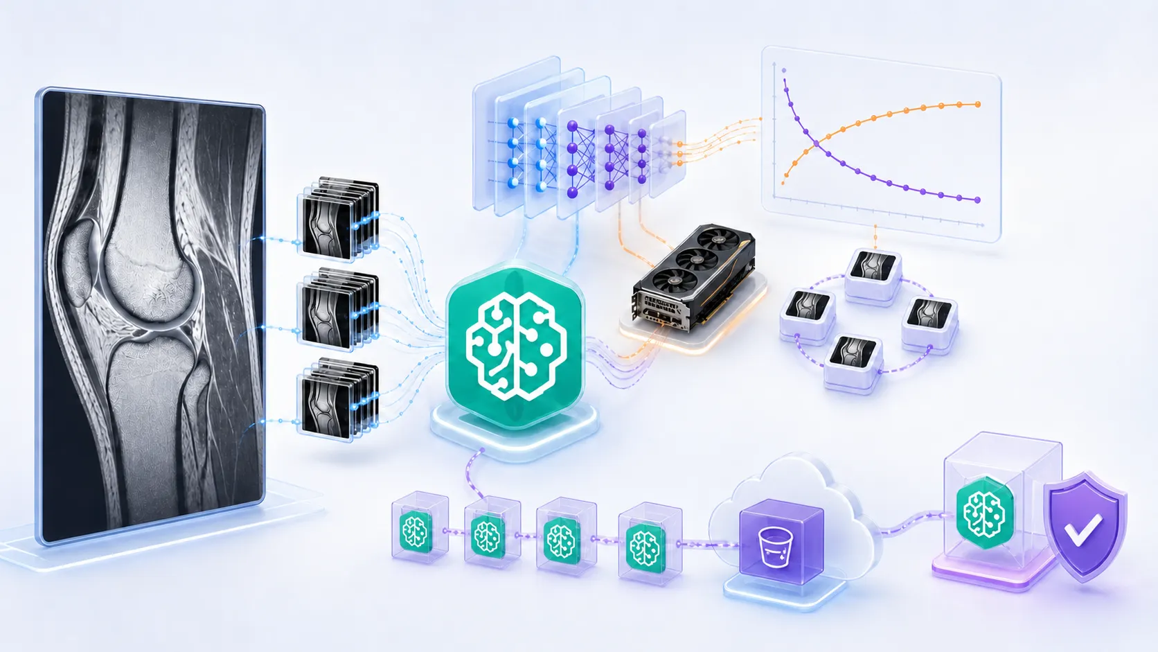
Building Trustworthy Knee MRI Training on AWS: Lessons from Amazon SageMaker AI
A field report on building a fold-safe, budget-aware knee MRI training system with Amazon SageMaker AI, Amazon S3, AWS KMS, CloudWatch, and AWS Budgets—and what an underperforming Kaggle submission taught me about honest validation.

My most useful training run was not my highest-scoring one.
It was the run that passed every engineering check, improved honest out-of-fold validation, completed an internet-disabled inference rehearsal, and then scored much lower on Kaggle than I hoped.
That result forced me to separate two ideas that are easy to conflate:
- a reproducible machine-learning system; and
- a model that generalizes well enough to win.
You need both, but the first does not guarantee the second.
This is the follow-up to my article about building an AWS-native ingestion pipeline for the RSNA Knee Abnormality Detection competition. Once the 247 GB compressed archive had become a validated, training-ready MRI cache, I moved the modeling workflow to Amazon SageMaker AI.
The task is multilabel classification of twelve knee abnormalities from MRI examinations. Reports are available during training, but inference must work from imaging data alone. The public leaderboard evaluates only part of the hidden test set, so reliable local validation matters more than repeatedly probing the leaderboard.
This article is not a winner's recipe. It is an honest field report about what worked, what failed, and how AWS helped make both outcomes useful.
Competition data remains subject to its own rules and license. The architecture below is reusable, but it does not include raw medical data, report text, credentials, patient identifiers, or private AWS resource names.
The training architecture
I deliberately kept the control plane small. Amazon S3 stores immutable inputs and durable outputs. SageMaker AI provides disposable GPU training. AWS KMS encrypts artifacts. Amazon CloudWatch captures logs. AWS Budgets and a local cost gate constrain launches.
1
2
3
4
5
6
7
8
9
10
11
12
13
14
15
16
17
18
19
20
Git commit + pinned container digest
                  |
                  v
       Fail-closed launch gate
       /      |       |       \
  Budget   Quota   Manifests   No active GPU job
                  |
                  v
       SageMaker ml.g5.2xlarge
       /        |          \
  S3 cache  weak labels  pretrained weights
                  |
                  v
  checkpoint + OOF predictions + run contract
                  |
                  v
       independent artifact audit
                  |
                  v
       next fold or stop decision
The most important property is that no training job is trusted merely because SageMaker reports
Completed. A job is accepted only after its output contract is independently validated.Lesson 1: Make paid compute the last step, not the first
My launcher is dry-run by default. Before SageMaker can create a paid job, it checks:
- the exact AWS account and Region;
- the current SageMaker quota;
- that no other project GPU job is active;
- the live AWS Budget state;
- a worst-case cost estimate with contingency preserved;
- the Git commit and source-bundle SHA-256;
- the training-container image digest;
- metadata, cache, weak-label, and pretrained-weight manifests;
- held-out-fold exclusions; and
- byte counts, checksums, and server-side encryption.
Only an explicit execution flag can cross that boundary.
This matters because AWS Budgets is an alerting and visibility mechanism, not a guaranteed hard stop. My project budget is USD 650, with USD 70 deliberately reserved as contingency. The launch code therefore uses the larger of the available actual and forecast cost signals and calculates the proposed job's worst-case cost before creating it.
At most one
ml.g5.2xlarge job is allowed at a time. This is both a cost policy and an experimental policy: one fold finishes, its artifacts are audited, and only then can the next fold begin.Why ingestion used m7i.4xlarge on-demand
The ingestion worker and the training worker solve different problems, so I did not use one instance type for both.
Ingestion ran on one Amazon EC2
m7i.4xlarge: 16 vCPUs and 64 GiB of memory, backed by a 2 TiB encrypted gp3 volume. M7i is a general-purpose family with a 4:1 memory-to-vCPU ratio, which fit a workload dominated by download, archive validation, DICOM parsing, decompression, hashing, and concurrent cache construction. Eight cache partitions ran as local CPU workers on that one instance. No GPU was paid for while the pipeline was performing storage and CPU work.I chose on-demand capacity for this stage because the 247 GB archive download and extraction were long, stateful operations. An interruption before the validated raw archive reached Amazon S3 would save little and complicate recovery. The worker instead had a 48-hour runtime backstop, a verified Mumbai-region price of USD 0.8484 per hour at the time of the run, a compute ceiling of USD 40.72, automatic termination, and
DeleteOnTermination=true for the temporary EBS volume. Prices vary by Region and date, so these numbers are evidence from this project rather than future quotations.The Amazon EC2 M7i instance page describes the family hardware. The practical lesson was simpler: reserve GPU capacity for tensor operations and use a CPU-and-storage-appropriate instance for preprocessing.
Why training standardized on ml.g5.2xlarge
The main SageMaker training profile uses one
ml.g5.2xlarge. Its underlying G5 size provides one NVIDIA A10G Tensor Core GPU with 24 GB of GPU memory, 8 vCPUs, 32 GiB of system memory, and up to 10 Gbps network bandwidth. Those specifications were a useful middle ground for this project: enough GPU memory for 336-pixel DINOv2-B/14 inputs with slice microbatching and activation checkpointing, without paying for a multi-GPU instance that the small labeled set could not use efficiently.Each job receives a 150 GiB training volume. Gradient accumulation turns one-study microbatches into a larger effective batch, while the model removes padded series before the visual encoder so GPU work is not wasted on padding. The Amazon EC2 G5 instance page provides the corresponding hardware table.
I briefly tested another single-GPU generation in a bounded pilot, but kept
ml.g5.2xlarge as the default. Changing instance family, container, model geometry, and optimization strategy at the same time would make both performance and cost comparisons difficult to interpret.How we actually used Spot and on-demand capacity
I requested quota for exactly one SageMaker managed-Spot
ml.g5.2xlarge and one on-demand ml.g5.2xlarge. The launcher selects Spot by default; --on-demand is an explicit reliability fallback.The early smoke tests, report folds, self-supervised folds, and first supervised cross-validation sequence used on-demand capacity. At that stage, predictable startup was more valuable than a potential discount: I was still debugging input contracts, memory use, and end-to-end artifacts. If a job failed, I wanted to know it was a code or data failure rather than a capacity event. The completed jobs'
BillableTimeInSeconds matched their training time, so I do not claim Spot savings for those runs.After the source, cache, checkpoint, and OOF gates stabilized, I moved the next expensive fold to managed Spot. The request sets
EnableManagedSpotTraining=true, writes recoverable state under /opt/ml/checkpoints, syncs that path to a fold-specific S3 checkpoint prefix, and gives the job a maximum wait time longer than its maximum runtime.That distinction matters:
- Maximum runtime bounds how long training may execute.
- Maximum wait time includes both waiting for Spot capacity and execution time.
- Checkpointing makes an interruption recoverable instead of forcing an epoch-zero restart.
In one live fold while drafting this article, SageMaker reported
InProgress / Starting with no TrainingStartTime. That was not a failed GPU and not yet a training charge; it meant the managed-Spot job was waiting for capacity. I left it untouched instead of launching a duplicate. According to the SageMaker managed-Spot lifecycle , a job can remain in Starting, enter Training, move through Interrupted, and later resume if capacity returns.The fallback policy is fail-closed: an on-demand replacement can launch only after the Spot job is terminal, the budget is rechecked, and no other project GPU job is active. We never race Spot and on-demand copies of the same fold.
AWS documents that Managed Spot Training can reduce cost substantially compared with on-demand capacity, but the realized saving must be measured after completion. SageMaker exposes
TrainingTimeInSeconds and BillableTimeInSeconds; the useful saving is calculated from those observed values, not from the headline maximum.Lesson 2: Immutable inputs turn debugging into evidence
Every run is identified by a Git commit, a pinned ECR image digest, an immutable metadata version, a cache manifest, and exact pretrained-weight hashes.
The S3 structure separates inputs from experiment outputs:
1
2
3
4
5
6
7
metadata/training-v1/
prepared/cache-v3/full-336/
prepared/pretrained/<model-revision>/
prepared/report-rubric-v1/fold-0/
experiments/image/fold-0/<job-name>/
checkpoints/image/<job-name>/
final/<candidate-version>/
Different preprocessing implementations never share a prefix. A 320-pixel cache and a 336-pixel physical-field-of-view cache are different datasets, even when they originate from the same DICOM files.
This discipline paid off when a model underperformed. I could answer:
- Which code produced the checkpoint?
- Which validation fold was excluded from weak supervision?
- Which pretrained revision initialized the encoder?
- Which geometry produced the tensors?
- Did the Kaggle notebook load the exact audited bytes?
Without immutable inputs, a disappointing score becomes guesswork. With them, it becomes an experiment.
Lesson 3: MRI geometry is part of the model
Knee MRI is not ordinary JPEG classification. Series can differ in orientation, pixel spacing, matrix shape, slice count, contrast, and left/right laterality.
My first cache normalized intensity and stored complete slice stacks, but later experiments made the spatial contract more explicit:
- read DICOM direction cosines and physical pixel spacing;
- order slices using image position and orientation;
- preserve a fixed physical field of view before resizing;
- canonicalize left and right knees into a consistent medial-lateral direction;
- avoid random horizontal flips, which can exchange medial and lateral anatomy; and
- sample neighbouring slices as 2.5D inputs.
For the stronger transformer experiment, the cache uses a 130 mm field of view and a 336-pixel input. The size is divisible by the DINOv2-B/14 patch size, which avoids silently changing the token geometry.
The same settings are embedded in cache objects and checkpoints. Training fails if the requested geometry disagrees with the cache. Offline inference reconstructs preprocessing from the checkpoint rather than from notebook defaults.
That is an MLOps lesson with a clinical consequence: a geometry mismatch can look like model drift even when the weights are unchanged.
Lesson 4: Validation leakage can enter through pretraining and reports
The fully labeled subset is small, so reports and unlabeled MRI examinations are valuable. They are also potential leakage paths.
I enforced a single rule:
Anything that learns from a study assigned to validation cannot initialize or supervise that fold.
For self-supervised MRI pretraining, I created one checkpoint per fold while excluding that fold's studies. The supervised trainer rejects a checkpoint whose
excluded_fold does not match the validation fold.For report supervision, raw reports never enter the image job. A rubric teacher converts training reports into soft probabilities for the twelve targets. Each fold receives only a fold-bound artifact whose gate proves that the held-out fold was excluded. Long-form report text and evidence excerpts are not written to the training artifact.
This costs more compute than training one universal representation, but it produces honest out-of-fold predictions. In a small medical dataset, that distinction is worth more than another decimal place from a leaky experiment.
Lesson 5: Weak supervision needs a controlled handoff to gold labels
My image model is hierarchical:
1
2
3
4
2.5D slices -> visual encoder -> slice attention
             -> series representation + acquisition descriptors
             -> target-specific study attention
             -> 12 abnormality probabilities
Training happens in stages:
- Head-only warm-up. The pretrained visual encoder is frozen while the new aggregation and classification layers learn a stable interface.
- Controlled unfreezing. Only the final transformer blocks are unfrozen, with a much smaller learning rate than the task-specific layers.
- Gold refinement. The best weak-stage checkpoint is reloaded and refined using original labels only, with conservative learning rates.
Model selection always uses gold validation labels. Pseudo-labels can increase training coverage, but they never enter the validation metric.
This schedule was introduced after observing that immediately fine-tuning the full backbone on noisy labels could erase useful pretrained features. Freezing forever was not ideal either. Staged unfreezing became the compromise.
Lesson 6: A five-fold score can still be uncertain
The first independently trained five-fold SSL image ensemble improved the pooled macro AUC from approximately 0.543 for the original image baseline to 0.635 on 58 fully labeled studies. A patient-level bootstrap produced a wide 95% interval of roughly 0.579 to 0.686.
That interval was the warning.
Fold-level macro AUC varied substantially. A report model and several blends were also evaluated. A full-fit blend reached a higher apparent score, but leave-one-fold-out meta-validation showed that the improvement did not survive. The defensible choice was therefore the simpler uniform mean of the five image folds.
The Kaggle result was 0.663. An earlier DINOv2 reference notebook had scored 0.809.
The submission was technically valid:
- all five checkpoints loaded strictly;
- output rows matched the competition order;
- all probabilities were finite and bounded;
- the notebook ran with internet disabled; and
- projected hidden-test runtime stayed below the nine-hour limit.
The model simply did not generalize as well as hoped.
This was not an infrastructure failure. It was a measurement lesson: five-fold cross-validation on 58 fully labeled studies can still have high variance and can still differ from the hidden test distribution.
Lesson 7: Preserve failed models; do not promote them
Deleting a weak checkpoint destroys information. Promoting it destroys trust.
Every SageMaker job emits:
- the selected checkpoint;
- exact out-of-fold predictions;
- training history;
- data and model configuration;
- source and artifact hashes; and
- a terminal run contract.
After download, an independent audit checks exact validation coverage, duplicate or missing studies, finite probabilities, strict state-dictionary loading, encryption, byte counts, and SHA-256 values.
A model can pass integrity and still regress. In that case, I preserve the artifact for per-target and diversity analysis, but I do not automatically spend money training the remaining folds.
That stop/go gate is one of the most valuable cost controls in the project.
Lesson 8: Optimize the complete inference system
The competition reruns a saved notebook against a hidden dataset with internet disabled and a nine-hour limit. Training accuracy is irrelevant if inference cannot finish.
The Kaggle package therefore contains all code and exact audited checkpoints. It does not download models at runtime.
The inference path also:
- reads all DICOM headers for physical ordering but decodes pixels only near sampled slice centers;
- shares decoded study tensors across compatible checkpoints;
- checks model keys and checkpoint configuration before prediction;
- writes runtime telemetry and a hidden-test projection;
- validates the exact submission schema and row order; and
- rejects missing, duplicate, extra, non-finite, or out-of-range predictions.
A three-study rehearsal completed in about 94 seconds and projected approximately 6.7 hours for the hidden test set. That left a meaningful safety margin under the competition limit.
SageMaker optimized training. The Kaggle notebook optimized delivery. Treating them as one system prevented a late surprise.
What AWS changed about my workflow
The biggest benefit was not access to a GPU. It was the ability to encode discipline into infrastructure:
| AWS service | Role in the workflow |
|---|---|
| Amazon S3 | Immutable datasets, manifests, checkpoints, OOF predictions, and final packages |
| Amazon SageMaker AI | Disposable, bounded, one-fold-at-a-time GPU training |
| AWS KMS | Encryption for source, inputs, checkpoints, and model artifacts |
| Amazon CloudWatch | Training logs and failure-stage evidence |
| AWS Budgets | Cost visibility and alerts used by the launch gate |
| AWS IAM | Prefix-scoped access for training and ingestion roles |
| Amazon ECR | Digest-pinned training container |
AWS did not make the model correct. It made every decision inspectable.
What I am changing next
The next experiment returns to the stronger DINOv2 family while keeping the validation and cost controls learned from the failed submission. It combines:
- physically normalized 336-pixel MRI inputs;
- canonical laterality;
- fold-safe rubric supervision;
- a head-only warm-up;
- selective unfreezing of the final backbone blocks; and
- lower learning rates for pretrained parameters.
The first fold is a decision gate, not a formality. If its artifact fails integrity or clearly regresses, the remaining folds will not launch. If it provides reasonable evidence, the same immutable configuration will continue sequentially across all five folds.
Only after exact-once OOF assembly, patient bootstrap analysis, and cross-fold stability checks will another Kaggle candidate be prepared.
Final takeaway
My main lesson from training medical-imaging models on AWS is simple:
Reproducibility does not guarantee generalization, but without reproducibility you cannot learn reliably from poor generalization.
Amazon SageMaker AI, Amazon S3, AWS KMS, CloudWatch, IAM, ECR, and AWS Budgets gave me a system where a failed leaderboard attempt still produced durable knowledge. The model can change. The evidence chain remains intact.
That is how I want to approach the next experiment—and every clinical machine-learning project after it.
# amazon-sagemaker-ai# machine-learning# computer-vision# healthcare-life-sciences-industry# amazon-s3
Any opinions in this article are those of the individual author and may not reflect the opinions of AWS.Enjoyed reading this content? Let the author know!
Your likes, comments, shares, and saves help creators reach more builders.

Loading recommendations
Loading article